A4: Sampling materials
In this assignment, we will take a deep dive into implementing a Monte Carlo renderer. Monte Carlo is a powerful technique for approximating integrals, and it is the dominant technique for rendering images in the movie industry and, increasingly, video games.
It turns out that the renderer you have been writing so far already did Monte Carlo integration in secret - but it was cleverly brushed under the table by Pete Shirley's books. In this assignment, you will redesign your renderer to make the Monte Carlo component explicit. This will allow you to implement much more powerful rendering techniques in the future.
This assignment consists of three parts. In the first, you will implement sampling routines for different distributions on the sphere. Then you will get to implement Monte Carlo sampling techniques for your existing materials. Finally, you will implement integrators that will allow you to render your scene with different rendering algorithms.
Task 1: Sampling distributions
In this task, you will start with the basics of generating points on the sphere that have specific distributions. We recommend you read Ray Tracing: The Rest of Your Life, Chapters 1-7, before you start.
To help you get a feel for what these different distributions look like, we want you to generate 3D visualizations of your point sets. For each of the distributions you will implement, write out a list of points to a text file and make a 3D scatter plot of the points. You can do this in Matlab or your favorite plotting software, or in one of many online plotting tools.
If you look at include/, you can see that we already provide you with two functions for generating points in a circle and points in a sphere. These are generated using rejection sampling as described in Pete Shirley's books. To help you get started setting up your plotting tools, generate a few hundred points using random_ and visualize them in your plotting tool. For reference, we will show you images of our points sets, which we generated by writing out a CSV file from C++ and rendering them using plot.ly (click on "import" to upload a CSV, and click on +Trace, type->3D Scatter to get a scatter plot). If you are familiar with Jupyter notebooks, we also include a short Python Jupyter notebook plot_csv.ipynb for convenience which allows you to do the same thing as the plot.ly website, but on your local computer with Python.
We generated the CSV by adding a new program in darts called point_gen with the following source code:
#include <darts/common.h>
#include <darts/sampling.h>

int main(int argc, char **argv)
{
    fmt::print("x,y,z\n");
    fmt::print("0,0,0\n");
    for (int i = 0; i < 500; ++i)
    {
        Vec3f p = random_in_unit_sphere();
        fmt::print("{},{},{}\n", p.x, p.y, p.z);
    }

    return 0;
}
To compile this new program, type your source code in a new <tt>.cpp file (we called it point_gen.cpp) and modify the main CMakeLists.txt file to tell your compiler about your new executable:
add_executable(point_gen src/point_gen.cpp)
target_link_libraries(point_gen PRIVATE darts_lib)
You can then run this program from the terminal as before.
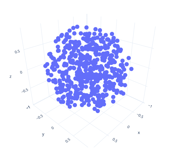
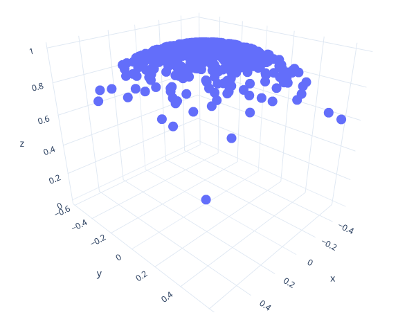
If you implemented everything correctly, your program should generate a point distribution like the one on the right.
This is only for inspiration: You don't have to do it this way, and are free to visualize your points in any way you want. Your output will differ depending on which plotting software you use, how many points you output and so forth, but it should look like uniform points within a sphere.
Avoiding rejection sampling
While rejection sampling will work, there are a couple issues with this design that will make it harder as we try to implement more sophisticated rendering techniques. Firstly, rejection sampling is generally undesirable since it can require an unknown amount of random numbers. The more serious problem is that this rejection sampling relies on randf() which is a global random number generator. Using a single global random number generator is a Very Bad Idea® if we have ambitions to ever introduce thread-level parallelism to our code (to render images more quickly by allowing the multiple cores on a single computer to trace the rays for different pixels simultaneously).
For these reasons, typical Monte Carlo renderers operate by creating a different random number generator per thread to provide each with its own endless stream of uniform random numbers. We'll do this part later on in this assignment. First, however, we'll move away from rejection sampling and instead sample each spherical distribution we are interested in using just a fixed and small number of uniform random numbers (typically 2).
We'll do this by implementing various functions of the form
Vec3f sample_<distribution>(const Vec2f & rv);
Each of these functions takes a random variable rv uniformly distributed in the unit square [0,1)2 domain and warps it to the desired distribution.
For each of these functions, we will also implement a corresponding
float sample_<distribution>_pdf(const Vec3f & v);
function that returns the PDF that the given direction v was sampled.
We already provide you with an example for a disk: sample_ and sample_.
Uniform points on the sphere
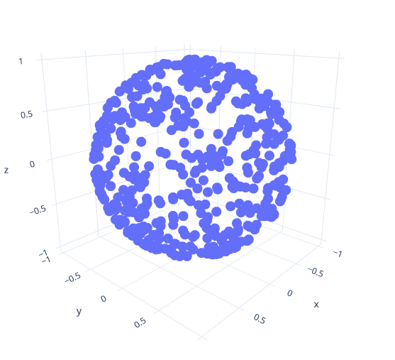
In include/, implement the function sample_ that generates points _on_ the sphere instead of its interior. You can begin by simply calling random_ and normalizing the result: That will project all points to the surface of the sphere, and give you a result like the one shown in the image.
While this gives you the distribution you want, we want to avoid rejection sampling and its use of randf(). WolframAlpha shows several ways to do this. The easiest is the trigonometric way we discussed in class, for which we give pseudocode below:
phi = 2*pi*<uniform random number>;
cos_theta = 2*<uniform random number> - 1;
sin_theta = sqrt(1 - cos_theta*cos_theta);
x = cos(phi)*sin_theta;
y = sin(phi)*sin_theta;
z = cos_theta;
return vector(x, y, z);
This requires two uniform random numbers. Instead of using randf(), you can instead use the provided uniform random variable rv, which contains both an x and a y component, each of which is a uniform random number. Note also that we provide a convenience function sincos in common.h which computes and returns both the sin and cos of an angle, and can sometimes lead to more optimized code.
Also implement the corresponding sample_ function. The samples are generated uniformly over the sphere, so this function should just return a constant value. But what value? To figure this out, remember that a PDF must integrate to 1 over the entire domain.
After you implement the functions without rejection sampling, rerun it and visualize the point set. It should give you the same distribution as before, except now you don't rely on rejection sampling.
Uniform points on the hemisphere
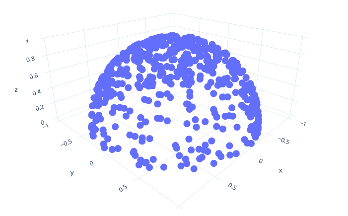
Implement the function sample_ (and the corresponding sample_) to generate points on the hemisphere (i.e. the parts of the sphere with positive z coordinated) instead of the full sphere. Hint: you can achieve this by modifying the way cos_theta is computed in the previous code for sampling the sphere to only produce positive z values.
Cosine-weighted points on the hemisphere
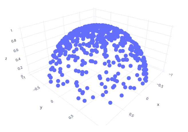
Implement the function sample_ (and the corresponding sample_). This function should generate points so that the PDF of the points is proportional to the cosine of the angle between the point and the z-axis. You can again achieve this by modifying the way you compute cos_theta in the previous functions: cos_theta = sqrt(<uniform random value>). This should give you a distribution like on the right.
Cosine-power-weighted points on the hemisphere
Add a new function called sample_hemisphere_cosine_power(float exponent) (and the corresponding sample_). This function should generate points so that the PDF of the points is proportional to the cosine of the angle between the point and the z-axis, raised to the power of some exponent. For an exponent of 1, we should get standard cosine-weighted hemisphere sampling; for an exponent of 0, we should get the uniform hemisphere, and the distribution should get more and more clustered around (0, 0, 1) for higher and higher exponents.
Yet again, you can achieve this by modifying the way you compute cos_theta in the above code. Change it to cos_theta = powf(<uniform random number>, 1/(exponent + 1)).
Try to insert exponent=0 and exponent=1 into the above equation. Does it do what we want it to do?
Write out a point set for exponent=20. This should give you a distribution as shown here. Note how clustered the points are around the z-axis.
Task 2: Sampling materials
In this task, you will redesign your Material class to support three new queries. The first of these is Material::eval(): This method will evaluate how much light flows between a given incoming and outgoing ray direction. This method entirely determines what the material will look like.
The other two queries are needed for rendering materials using Monte Carlo. The Material::sample() method takes an incoming ray direction and samples an outgoing ray direction. The Material::pdf() function returns the probability density of the ray directions produced by Material::sample(). These two queries need to be exactly matched to each other - i.e. Material::pdf() should actually be the exact distribution of samples coming out of Material::sample() – but they do not have to match the shape of the material reflectance exactly (i.e. Material::pdf() does not have to match Material::eval()). It helps if it does – you will have less noise that way — but it does not have to. This allows you to render materials that cannot be sampled exactly. This is a big departure from Peter Shirley's books, in which it is implicitly assumed that the sampling method matches the material reflectance exactly, and changing the Material:: method would change both the sampling strategy and the appearance of the material.
Begin by adding new virtual methods for each of the three queries to the Material base class in include/. You can design these any way you would like, but to help you get started, we give you the interfaces we use in our code for inspiration:
/*
    Evaluate the material response for the given pair of directions.

    For non-specular materials, this should be the BSDF multiplied by the
    cosine foreshortening term.

    Specular contributions should be excluded.

    \param  wi         The incoming ray direction
    \param  scattered  The outgoing ray direction
    \param  hit        The shading hit point
    \return Color3f    The evaluated color
*/
virtual Color3f eval(const Vec3f &wi, const Vec3f &scattered, const HitInfo &hit) const
{
    return Color3f(0.0f);
}

/*
    Sample a scattered direction at the surface hitpoint \p hit.

    If it is not possible to evaluate the pdf of the material (e.g.\ it is
    specular or unknown), then set \c srec.is_specular to true, and populate
    \c srec.wo and \c srec.attenuation just like we did previously in the
    #scatter() function. This allows you to fall back to the way we did
    things with the #scatter() function, i.e.\ bypassing #pdf()
    evaluations needed for explicit Monte Carlo integration in your
    #Integrator, but this also precludes the use of MIS or mixture sampling
    since the pdf is unknown.

    \param  wi     The incoming ray direction
    \param  hit    The incoming ray's intersection with the surface
    \param  srec   Populate \p srec.wo, \p srec.is_specular, and \p srec.attenuation
    \param  rv     Two random variables in [0,1) to use when generating the sample
    \return bool   True if the surface scatters light
*/
virtual bool sample(const Vec3f &wi, const HitInfo &hit, ScatterRecord &srec, const Vec2f &rv) const
{
    return false;
}

/*
    Compute the probability density that #sample() will generate \c scattered (given \c wi).

    \param  wi         The incoming ray direction
    \param  scattered  The outgoing ray direction
    \param  hit        The shading hit point
    \return float      A probability density value in solid angle measure around \c hit.p.
*/
virtual float pdf(const Vec3f &wi, const Vec3f &scattered, const HitInfo &hit) const
{
    return 0.0f;
}
You can see that Material::sample() does not return the scattered direction, but instead fills out a ScatterRecord structure. Our structure looks as follows:
struct ScatterRecord
{
    Color3f attenuation;         // Attenuation to apply to the traced ray
    Vec3f   wo;                  // The sampled outgoing direction
    bool    is_specular = false; // Flag indicating whether the ray has a degenerate PDF
};
This might look strange: In theory, all that Material::sample() needs to generate is a scattered direction. However, there are two additional fields: ScatterRecord::attenuation and ScatterRecord::is_specular. The reason for this is that certain materials (like mirrors or glass) do not have real PDFs, or have PDFs that are very difficult to compute (like Peter Shirley's metal material).
For now, implement the Material::sample() method for all your existing materials and make it a) set ScatterRecord::is_specular to true – signaling to the rest of the code that this material does not have a PDF and we should fall back to the non-Monte Carlo way of computing colors, and b) fill out ScatterRecord::wo and ScatterRecord::attenuation by doing something just like in the Material:: method (though without rejection sampling or the global randf()). This fallback will make sure your existing materials are backwards compatible. In the following tasks, you will slowly replace the fallback with real sampling code and PDFs.
Lambertian sampling
The formula for the Lambertian material is extremely simple: It only depends on the normal and the scattered direction, and does not take the incoming direction into account. In pseudo-code, it is albedo * max(0, dot(scattered_dir, normal))/pi. Implement this as the Lambertian::eval() method.
The PDF of a Lambertian material is even simpler: It is max(0, dot(scattered_dir, normal))/pi. Implement this as the Lambertian::pdf() method.
The only remaining problem is to sample this PDF. However, you already implemented the bulk of the sampling code in Task 1, when you implemented sample_. All you need to do is to modify the Lambertian::sample() method to set srec.wo to the random cosine-weighted direction. Since you now have proper sampling code, remember to set is_specular to false!
Testing your code
Testing sampling code can be notoriously difficult. To help you with this, we added a new sampling test into darts in src/tests/material_. Add this to the list of sources for darts_lib in the CMakeLists.txt file. Note that this code assumes you use the same sampling interface as we use – if you made changes, you might have to adapt the tool.
Once you get the new code compiled, run darts scenes/assignment4/test_materials.json.
The tester will do two things: First, it will evaluate Material::pdf() over the sphere and output its integral. This integral should be close to 1 (otherwise, it is not a PDF). You should see an output like:
Integral of PDF (should be close to 1): 1.00003
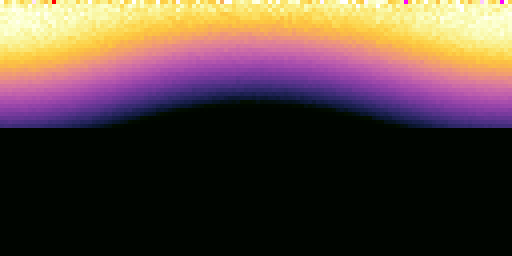
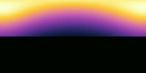
Second, the code will call Material::sample() many times and build a histogram of the sampled directions. This histogram should exactly match the PDF. The tester will output two images, lambertian-pdf.png (the PDF) and lambertian-sampled.png (the histogram). These should match with each other and look similar to this:

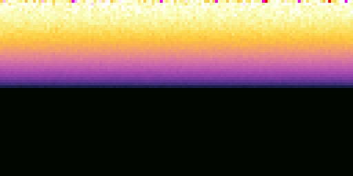
Additionally, your sample method should return successfully and not generate invalid directions; the code will test for that and output a statement like
100% of samples were valid (this should be close to 100%)
Make sure your code passes the tests before proceeding. If you have any problems, make sure you normalize the directions that are passed into your code – sometimes the scattered/dir_in directions might not have unit length, which will make your code misbehave.
Oriented samples
So far, your Lambertian sampling code has a big problem: It assumes the normal is (0, 0, 1). This makes the sampling algorithm simpler, but – of course – most of the time, the surface normal will not be (0, 0, 1).
To fix this, read Chapter 8 of the text book and implement an ONB (Ortho-Normal Basis) class. This will allow you to rotate directions for arbitrary normals. Modify your Material::sample() code to transform the sampled direction from sample_ using the ONB, oriented to the surface normal. You can look at Peter Shirley's code for inspiration.
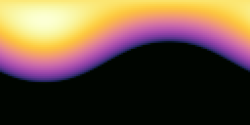
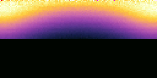
You can test your code using the "rotated-lambertian" test in the sample test scene. You should get images like these:

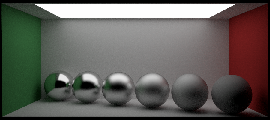
Phong material
Next to Lambert, the Phong reflection model is one of the earliest and simplest in computer graphics. It tries to model glossy reflections, such as from rough metal or plastic. Start by adding a new material class in src/materials/phong.cpp called Phong.
To allow our JSON parser to recognize this new type of Material, we need to inform it how to create a Phong material and which type string ("phong") to associate with it. Calling the following macro at the bottom of src/materials/phong.cpp will accomplish what we want:
DARTS_REGISTER_CLASS_IN_FACTORY(Material, Phong, "phong")
For a perfect mirror material (such as polished metal), all light scatters into the mirror direction, i.e. the incoming ray reflected by the normal. The Phong material tries to approximate surface roughness by "blurring" the reflection direction about the perfect mirror direction. The amount of spread can be controlled by a parameter to model different amounts of roughness of the surface. In the Phong material, this spread is called the exponent. Add an exponent member to your Phong class, and get it from JSON in the Phong constructor.
The PDF of the Phong material looks like this (pseudocode):
mirror_dir = normalize(reflect(dir_in, normal));
cosine = max(dot(normalize(scattered), mirror_dir), 0);
return constant*powf(cosine, exponent);
It measures the cosine of the angle between the scattered direction and the perfect mirror direction. The cosine is then raised to a power. For low exponents, there is a wide spread of this PDF around the mirror direction; for large exponents, the PDF becomes more and more concentrated around the mirror direction. constant is a normalization constant to make sure the PDF integrates to 1. It is computed like this: constant = (exponent + 1)/(2*pi).
The result of Phong::eval() is simply the PDF multiplied by the albedo.
Sampling this material follows in two steps:
First, you need to generate directions from a distribution proportional to a cosine raised to a power (Hint: You already implemented this; it is sample_hemisphere_cosine_power(exponent)). Second, you need to orient those samples so they are centered on the mirror direction (Hint: Use your ONB class, centered on the reflected incoming direction). Note that this can generate directions below the hemisphere, so make sure to reject those (i.e. return false in Phong::sample())!
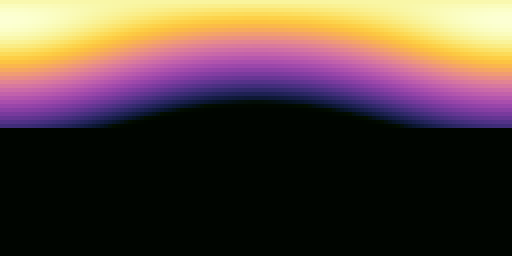
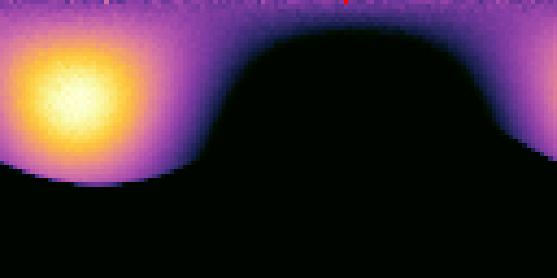
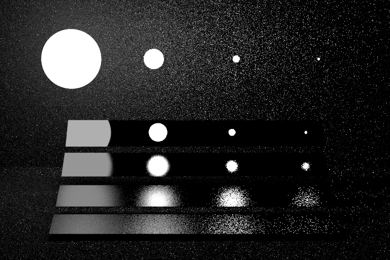
You can test your code using the "phong" and "rotated-phong" tests in the sample test tool. You should get images like these:

Grad students only: Blinn-Phong
If you are a grad student, you will also need to implement the _Blinn-Phong_ shading model, which is a slightly more realistic variation on the standard Phong model. In Blinn-Phong, we first generate a random normal, and then treat that normal as the surface normal for reflecting the incoming direction. Similar to Phong, this will create random directions distributed around the mirror direction, but with a different shape. Begin by creating a new BlinnPhong material that also has an exponent parameter, just like Phong. Use our DARTS_REGISTER_CLASS_IN_FACTORY macro to create this new material for the "blinn_phong" key.
The easiest method to implement is the BlinnPhong::sample() method, which we will start with. It should use sample_ and your ONB class to generate a cosine-power weighted direction centered on the surface normal. Use this new, random direction to reflect the incoming ray (as if the random direction was the real surface normal). Note that this can generate directions below the hemisphere, so make sure to reject those (i.e. return false in BlinnPhong::sample())!
The PDF method will be slightly more complicated. You first need to figure out which random normal would reflect the (given) incoming ray so that it matches the scattered ray. You can use the fact that the normal must lie exactly halfway between the incoming and scattered direction:
random_normal = normalize(-normalize(dir_in) + normalize(scattered))
Then, you need to compute the PDF of generating this random normal. Since we generated this from a cosine-power distribution, this must be the cosine-power PDF:
cosine = max(dot(random_normal, real_normal), 0);
normal_pdf = (exponent + 1)/(2*pi) * powf(cosine, exponent);
Finally, we need to account for a warping of the PDF by the reflection operation. The final PDF becomes:
final_pdf = normal_pdf/(4*dot(-dir_in, random_normal))
The BlinnPhong::eval() method is simply the PDF method times the albedo.
You can test your implementation using the sample tester tool. You should get images like these:

Task 3: Samplers
As mentioned previously, one of our goals is to move away from using the global random number generator in randf(), and instead create an explicit random number generator (it then becomes much easier to parallelize our code where each thread maintains its own random number generator). In rendering we typically call this abstraction a Sampler instead of a random number generator, partially because it produces samples for the Monte Carlo algorithm, but also because we can create Samplers that don't actually produce pseudo-random numbers at all, but rather carefully crafted deterministic samples that can often compute lower noise images more quickly.
We provide a base class for all Samplers in include/, as well as a default example Sampler in src/ which just generates independent random samples. Go read the implementation and comments in these two files to get an overview. You'll notice that we use our DartsFactory mechanism and the DARTS_REGISTER_CLASS_IN_FACTORY macro to allow the scene to specify a specific sampler type by name. We won't be implementing different types of Samplers in this assignment, but you now have a nice framework to explore this for your final project if you want.
We do need to introduce a small change to our parser to make this work. First, add a new member variable to Scene in include/: shared_ptr<Sampler> m_sampler;. Then, where we currently have a block of code in Scene:: that starts with:
//
// read number of samples to take per pixel
//
...
you'll need to replace it with something like:
//
// parse the sampler
//
if (j.contains("sampler"))
{
    json j2 = j["sampler"];
    if (!j2.contains("type"))
    {
        spdlog::warn("No sampler 'type' specified, assuming independent sampling.");
        j2["type"] = "independent";
    }
    m_sampler = DartsFactory<Sampler>::create(j2);
}
else
{
    spdlog::warn("No sampler specified, defaulting to 1 spp independent sampling.");
    m_sampler = DartsFactory<Sampler>::create({{"type", "independent"}, {"samples", 1}});
}
This allows our code to be backwards compatible with our previous scene files which have no concept of a Sampler, while allowing you to explore different samplers in the future.
Task 4: Integrators
In this task, you will extend your renderer to support different _integrators._ In computer graphics, we say "integrator" to refer to an algorithm for rendering an image. So far, we have been using the algorithm outlined in Peter Shirley's books, but there are more powerful (and less noisy) integrators out there, and you will implement the ability to select different integrators in this task.
Begin by creating an Integrator base class (you could do this in a new header file called include/darts/integrator.h. This class should have a method for returning the color along a particular ray similar to Scene:: that we used in previous assignments. You can call this method what you would like, but we named it Integrator::Li() for "Incoming radiance" or "light, incoming". You can add parameters to this method as you see fit, but it will need access to our recently introduced Sampler. For inspiration, this is what our method looks like:
/*
    Sample the incident radiance along a ray

    \param scene    The underlying scene
    \param sampler  A sample generator
    \param ray      The ray to trace
    \return         An estimate of the radiance in this direction
*/
virtual Color3f Li(const Scene &scene, Sampler &sampler, const Ray3f &ray) const
{
    // The default integrator just returns magenta
    return Color3f(1, 0, 1);
}
Normal integrator
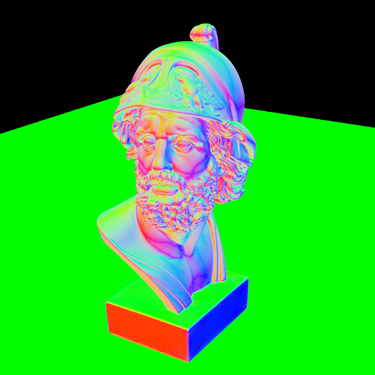
To test your new integrator class, create a test integrator class called NormalsIntegrator that inherits from Integrator and simply renders the normals of the visible geometry in the scene. In NormalsIntegrator::Li(), call scene.intersect() to intersect the scene along the ray passed to Li and, if you hit something, return the absolute value of the shading normal as the output color. If you do not hit anything, return black. Since we will ultimately support many different types of integrators, we organized our new source file under src/integrators/normals.cpp.
Now that we have a test integrator, we need to do some plumbing to make the scene use our new integrator interface. In the Scene class (in include/), add a shared_ptr<Integrator> m_integrator; field. This will contain the integrator used for rendering the image. Go to scene.cpp and change Scene:: to call m_integrator->Li(*this, ...) instead of Scene::. To remain backwards compatible with scenes files that don't specify an integrator, you could first check if m_integrator is null, and use the old Scene:: if it is.
Now let's add the ability to set the integrator from JSON. In parser.cpp, go to Scene::. Take inspiration from the way Scene:: sets the accelerator of the scene. Add some code that checks for an "integrator" field and sets the m_integrator member of the scene. We want to support many different kinds of integrators, so we'll use the DartsFactory<Integrator>::create() function that uses the "type" field of the JSON object to automatically create the appropriate integrator.
To make this work, we also need to inform the DartsFactory how to create the new integrator and which type ("normals") to associate with it. To do this, add the following macro at the bottom of src/integrators/normals.cpp:
DARTS_REGISTER_CLASS_IN_FACTORY(Integrator, NormalsIntegrator, "normals")
You can now test your implementation by running it on scenes/assignment4/ajax-normals.json. If everything works correctly, you should get an image like this:
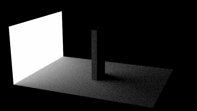
Ambient occlusion integrator
Now that the machinery for different integrators is in place, we can start creating more interesting integrators. Create a new AmbientOcclusionIntegrator class that will generate an ambient occlusion image.
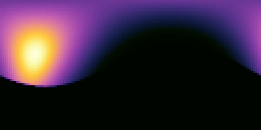
Ambient occlusion is a rendering technique which assumes that a (diffuse) surface receives uniform illumination from all directions (similar to the conditions inside a light box), and that visibility is the only effect that matters. Some surface positions will receive less light than others since they are occluded, hence they will look darker.
Implementing ambient occlusion is very simple: In your integrator's Li method, first find the intersection along the passed in camera ray. If the ray misses the scene, return black; if it hits a surface, sample the material at that point (use your new sample method for this). Now, construct a new "shadow" ray starting at the hit location going in the scattered direction, and check if it intersects something. If this new ray does not intersect anything, it means this ray sees the white "sky": Return white in this case. If the ray hits something, the sky is occluded, and you should return black instead. We put our implementation in src/integrators/ao.cpp.
Make sure to register the new integrator with the DartsFactory by adding
DARTS_REGISTER_CLASS_IN_FACTORY(Integrator, AmbientOcclusionIntegrator, "ao")
to the bottom of your implementation file. Because we rely on the DartsFactory in the parser, it should now automatically create either a normals integrator or an ambient occlusion integrator, depending on the "type" field of the "integrator" JSON object in the scene file.
You can test your implementation by running it on scenes/assignment4/ajax-ao.json. If everything works correctly, you should get an image like this:
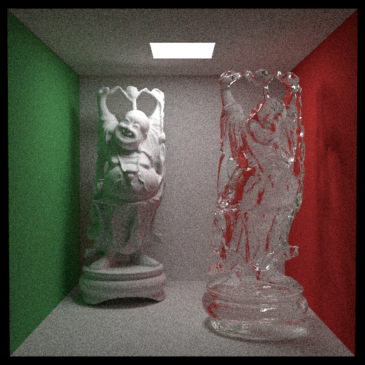
Material sampling integrator
The algorithm described by Peter Shirley in his books is (secretly) a form of path tracing, which is a rendering algorithm that traces rays exclusively from the camera. The flavor of path tracing you have been implementing in the previous assignments is sometimes called "Kajiya-style path tracing", after its inventor.
In this task, you will reimplement this flavor of path tracing as its own integrator, but this time you will make the PDFs and sampling methods that are involved explicit. This will allow you to implement more powerful forms of path tracing in the future.
Begin by making a new PathTracerMats integrator. We put ours in src/integrators/path_tracer_mats.cpp. This integrator will start from a camera ray and recursively trace new rays by sampling materials. Write your Li method based on the Scene:: method you wrote in previous assignments. Instead of calling Material:: and multiplying recursive calls by attenuation, call your new Material::sample() method, and multiply recursive calls by Material::eval() and divide by Material::pdf(). Implicitly, that is what Peter Shirley's algorithm was already doing: attenuation was eval/pdf in disguise, with factors appearing in both terms already cancelled out.
The only wrinkle in this is that some materials might not support the PDF interface (such as mirrors/glass or Peter Shirley's metal material). You can detect this by checking the is_specular flag; if that is set, multiply by attenuation instead of eval/pdf.
Make sure to also read in the "max_bounces" JSON field and limit your recursion to that depth. "max_bounces": 1 should result in direct illumination.
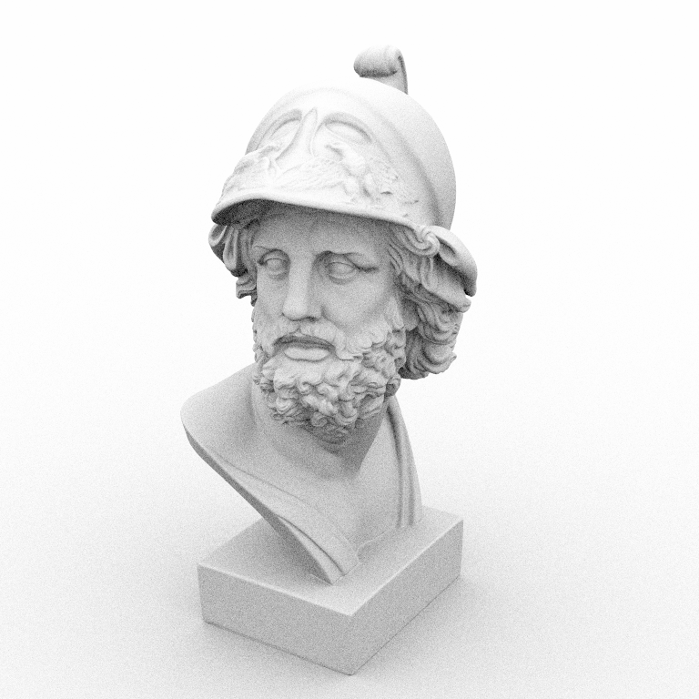
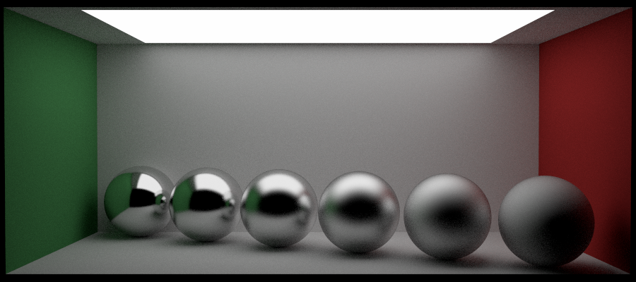
You can test your implementation by rendering the remaining scenes in scenes/assignment4. We show the results from our implementation below. You can further test your code by re-rendering some of the scenes from previous assignments using your new integrator-based implementation.
What to submit
In your report, make sure to include:
- Visualized point sets for all distributions from task 1
- Rendered images of all the scenes in
scenes/assignment4
Then submit according to the instructions in the Submitting on Canvas section of Getting started guide.